Everything You Need to Know About MTF Curves: From Misunderstanding to Practical Application
I. Do You Buy Lenses In This Way?
What research do you conduct before purchasing a lens? Chances are, you search for reviews online, browse a few sample images, glance at the price — and then place your order.
But if you’re a rational consumer, you’ve probably taken one extra step: Open the manufacturer’s official website, locate the MTF curve, stare at it for three seconds… and then close the page.
Why? Because you don’t understand it. Or worse — you think you understand it, but you’ve actually misinterpreted it.
This isn’t meant to mock anyone. Misreading MTF curves is almost an unspoken norm in the industry. Today, we’ll break down this graph completely. By the end of this article, you’ll discover it holds far more insights than you might expect.
II. A Memorable Case of Misjudgment
A few years ago, our team was selecting industrial inspection lenses and had to choose between two options with similar focal lengths and price points.
Lens A: Its MTF curve starts at an exceptionally high level. The central field delivers outstanding performance at both 10 lp/mm and 30 lp/mm, appearing nearly “perfect” at a glance.
Lens B: Slightly inferior to Lens A at the center, yet it maintains much more stable performance at the field edge, with a smaller gap between the two characteristic curves.
Nearly all our engineers leaned toward Lens A — simply because its numerical values were higher.
However, real-world testing revealed that Lens B performed better in our inspection scenarios. It offered more uniform edge image quality, free from the obvious “sharp center, blurry edge” discrepancy seen with Lens A, and maintained a more consistent detail recognition rate.
In our post-analysis, we realized we’d only focused on “how high the curves were” while completely overlooking several critical pieces of information hidden in the curve — one of which is even tied to the physical limits of optical imaging.
III. What Exactly Does an MTF Curve Tell Us?
1. First, let’s grasp the essence: What does MTF actually measure?
MTF stands for Modulation Transfer Function. Many people have memorized this term, yet few truly understand what it quantifies.
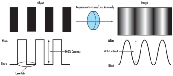
Let’s use an intuitive thought experiment: Imagine a pattern of alternating black and white zebra stripes. The denser the stripes, the higher the spatial frequency. Place this pattern in front of a lens and capture it with an image sensor.
You’ll notice: The denser the stripes, the less distinct the black and white tones appear in the captured image — the contrast gradually decreases. MTF is precisely the function used to quantify this loss of contrast.
2. Diffraction-Limited MTF — The "Ceiling Line" You Rarely Notice
This is a step skipped by 99% of MTF tutorials, yet it contains one of the most valuable pieces of information.
Every lens — even one with perfect manufacturing and zero aberrations — has a theoretical performance limit determined by diffraction.
For a circular aperture, the cutoff frequency of diffraction-limited MTF is defined as:

Take λ = 550 nm and F/2.8 as an example:

On the normalized frequency axis, the shape of the diffraction-limited MTF curve approximates an inverse cosine function — it declines smoothly from a high value at low frequencies to zero at the cutoff frequency.
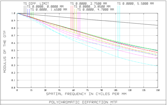
So what does the gap between this "ceiling line" and the actual MTF curve really mean?
| Gap Magnitude |
Meaning |
| Actual curve closely follows the diffraction limit |
Extremely low aberration, close to diffraction-limited design, with top-tier manufacturing process |
| Close to the limit at mid and low frequencies, obviously lower at high frequencies |
Residual aberrations (such as spherical aberration, coma) have a significant impact in the high-frequency range |
| Large deviation from the limit across all frequencies |
Excessive optical aberrations, unoptimized optical design, or manufacturing defects of the lens sample |
| Actual curve exceeds the diffraction limit in certain frequency bands |
Questionable data — possibly caused by improper testing methods or artificial curve modification |
The actual MTF curve can never exceed the diffraction-limited MTF at the same aperture. If you see a lens whose MTF curve rises above the diffraction limit in any frequency range, it is either due to inconsistent test conditions or flawed data.
This is extremely critical for industrial lens acceptance. Using the diffraction-limit curve as a reference enables objective evaluation of a lens’s design quality, rather than relying solely on empirical judgments like “any MTF value above 0.8 is good enough”.
3. Identify Main Aberration Types from MTF Curves
This is the advanced way to read MTF charts. Different optical aberrations leave unique “fingerprints” on the MTF curve.
Spherical Aberration
Characteristics: Overall central MTF is relatively low; the curve begins to decline even at low frequencies and changes significantly with aperture adjustments.
-
For lenses with severe spherical aberration, the central MTF at wide-open aperture is noticeably lower than when stopped down by two stops.
-
Positive spherical aberration causes asymmetric MTF performance before and after the focal plane — higher MTF at the front focal plane and lower at the rear, or vice versa.
Practical Judgment: If the same lens shows a significant MTF difference (especially at the center) between f/1.4 and f/5.6, spherical aberration is the primary culprit.
Coma
Characteristics: At moderate field heights, the Sagittal (S) and Tangential (T) curves cross or exhibit abnormal fluctuations.
-
Coma is usually most noticeable in the mid-field area, not at the extreme edge.
-
A point light source (such as a star) will produce a “comet tail” when coma is severe.
Practical Judgment: If your MTF curve shows an abnormal “rise-then-fall” pattern at 0.3–0.5 field height, coma should be your first suspect.
Astigmatism
Characteristics: The Sagittal and Tangential lines (solid and dashed lines) separate, and the gap between them widens as field height increases.
-
When astigmatism dominates, the S and T lines bend in opposite directions.
-
Result: Radial and tangential lines exhibit inconsistent sharpness.
Practical Judgment: Astigmatism is the easiest aberration to identify from an MTF chart. The larger the gap between the two lines and the faster it widens with field height, the more severe the astigmatism.
Field Curvature
Characteristics: The S and T lines decline synchronously with little separation, yet both drop rapidly as field height increases.
-
Lenses with significant field curvature feature a sharp center but blurry edges; both curves remain low but close to each other.
-
Key difference from astigmatism: Astigmatism causes the lines to separate, while field curvature causes both lines to drop together.
Practical Judgment: If both edge curves are low but closely aligned, field curvature is more significant than astigmatism. Such lenses struggle with flat-plane shooting scenarios, such as document scanning or copying.
Distortion
MTF curves cannot directly reflect distortion. Distortion affects geometric positioning, not contrast transfer. This is one of the most well-known blind spots of MTF.
|
Aberration Type
|
MTF Curve Characteristics
|
Affected Area
|
|
Spherical Aberration
|
Low central MTF, highly sensitive to aperture
|
Entire field of view, mainly the center
|
|
Coma
|
Abnormal fluctuation of S/T curves at middle field
|
Moderate field height
|
|
Astigmatism
|
Obvious separation between Sagittal and Tangential curves
|
Mid-field to edge field
|
|
Field Curvature
|
S/T curves decline synchronously with field height and remain closely aligned
|
Mainly edge field
|
|
Distortion
|
Cannot be reflected by MTF
|
—
|
I. Center vs Edge vs Full Field — Three‑Segment Analysis Method
When reading MTF curves, we recommend dividing the field of view into three segments, each with a distinct focus:
Central Area (0–0.3 Field Height)
Key concerns: Spherical aberration, upper limit of optical design performance
-
The height of the curves here reflects the lens’s absolute optical capability.
-
Comparison with the diffraction limit: The smaller the gap, the closer the design is to the physical limit.
-
The Sagittal and Tangential curves should nearly overlap here. If they are already separated at the center, it indicates insufficient correction of on-axis aberrations.
Design tip: Focus on high-frequency curves (e.g., 30 lp/mm or even 50 lp/mm), as these truly reflect central resolution performance.
Edge Area (0.7–1.0 Field Height)
Key concerns: Astigmatism, field curvature, distortion (to be checked separately)
-
The gap between the S and T curves is largest here — the area where astigmatism is most prominent.
-
If both curves are low but closely aligned, field curvature dominates; if the two curves are widely separated, astigmatism is the main issue.
-
High-demand scenarios (such as full-frame astrophotography and full-target industrial machine vision inspection) have extremely strict requirements for this segment.
Design tip: Judge whether requirements are met based on the absolute MTF value at the edge, not just how much lower it is compared to the center.
Middle Area (0.3–0.7 Field Height)
Key concerns: Coma, astigmatism transition, field flatness
-
This is the most easily overlooked area and a common location for coma.
-
Abnormal bulges or crossovers in the curve here should first prompt a check for coma.
-
A smooth transition from the central to edge curve reflects the maturity of the overall field design.
Design tip: Observe the overall trend across the three segments. A “high-flat-slightly lower” pattern (strong center → stable middle → mild drop at the edge) is typical of a well-optimized lens design.
Comprehensive Skills for Full‑Field Analysis
Create an S-T separation heat map: Mentally or on paper, mark the S-T gap at different field heights. The location with the largest gap is where aberrations are concentrated. For engineering acceptance, this method is far more valuable for locating issues than simply checking individual MTF values.
5. Test Conditions — Read the Fine Print Before Interpreting the Chart
The “birth certificate” of an MTF curve is often hidden in the chart’s footnotes:
Maximum aperture vs Optimum aperture
Many manufacturers only display MTF performance at the optimum aperture (typically f/5.6–f/8), not at the maximum aperture. The difference between the two can be substantial.
Design value vs Measured value
Some manufacturers provide theoretical simulation data from Zemax, not actual measured results. Theoretical values tend to be overly optimistic and do not account for manufacturing tolerances or assembly errors.
White light vs Monochromatic light
White light testing includes the effects of chromatic aberration; monochromatic light testing eliminates chromatic aberration, resulting in higher MTF values that do not represent real-world white-light imaging performance.
6. Advanced: Information That MTF Curves Cannot Reveal
While MTF curves are powerful tools, they inherently have blind spots.
|
Information Type
|
Can MTF Tell You?
|
Alternative Method
|
|
Central resolution and contrast
|
✅
|
—
|
|
Magnitude of astigmatism
|
✅ (Check separation between S/T curves)
|
—
|
|
Field flatness
|
✅ (Check curve slope)
|
—
|
|
Estimation of spherical aberration / coma
|
✅ (Indirect judgment)
|
Combine with spot diagram
|
|
Distortion
|
❌
|
Dedicated distortion test
|
|
Chromatic aberration (purple fringing / green fringing)
|
❌
|
LCA curve analysis or sample imaging
|
|
Ghosting / flare
|
❌
|
Dedicated stray light test
|
|
Bokeh texture and out-of-focus quality
|
❌
|
Actual shooting sample evaluation
|
|
Mechanical reliability, dustproof and waterproof performance
|
❌
|
Specification sheet + physical testing
|
MTF is a necessary condition but not a sufficient condition for lens selection and acceptance inspection.
Now, let’s take a quick quiz:
Given the two MTF curves below, which lens would you choose?
Lens A: 10 lp/mm MTF = 0.95, 30 lp/mm MTF = 0.85; central performance is close to the diffraction limit. However, the gap between the Sagittal and Tangential curves widens significantly toward the edge, with a separation of approximately 0.3.
Lens B: 10 lp/mm MTF = 0.88, 30 lp/mm MTF = 0.75; the center has a noticeable gap from the diffraction limit. Yet the S/T curves remain closely aligned across the entire field, with an edge separation of less than 0.05.
If your applications include street portrait photography, architectural panoramas, or full-target industrial vision inspection — choose Lens B. Uniform image quality and excellent astigmatism control are more critical in these scenarios.
If you mainly shoot central-subject portraiture with large-aperture blurred backgrounds — Lens A is perfectly suitable, offering stronger central sharpness.
There is no absolute “good” or “bad” lens — only suitability for your specific application.
IV. What Is the MTF Acceptance Standard in Your Company?
After covering all these fundamentals, here’s a thought-provoking question for everyone:
What MTF acceptance standard does your company or project use for lens incoming inspection?
-
Is it MTF ≥ 0.3 at 30 lp/mm, or MTF ≥ 0.5 at 50 lp/mm?
-
Do you set separate criteria for the center and edge of the field?
-
Is the test conducted under white light or monochromatic light?
-
Do you benchmark the actual MTF against the diffraction limit curve?
Acceptance standards vary greatly across industries and application scenarios. Consumer photography, industrial machine vision, medical imaging, aerospace remote sensing — each field has its own performance baseline.
Feel free to share your internal standards in the comments. I will compile them into an industry comparison table. This real-world data will be far more valuable than any ordinary lens review.
